14 Parallel Algorithms
1 Introduction#
- Machine parallelism
- multiple processors
- pipelning
- Very-Long Inst Word (VLIW)
- Parallel algorithms
1.1 Models#
- Parallel Random Access Machine (PRAM) 并行随机访问机
- Work-Depth (WD) 工作深度
1.2 Basic concepts#
- Unit time, 读写计算的操作都简化为单位时间
- Shared memory, 所有处理器都使用同一块内存
2 Conflicts#
| step2\1 | R | W |
|---|---|---|
| R | no | conflict |
| W | no | conflict |
2.1 Exclusive-Read Exclusive-Write (EREW)#
- 完全不允许同时读写
2.2 Concurrent-Read Exclusive-Write (CREW)#
- 同时读,分开写
2.3 Concurrent-Read Concurrent-Write (CRCW)#
- 同时读,同时写
- 同时写冲突解决
- Arbitrary rule
- Priority rule: 每个处理器分配一个权重,写入优先级高的
- Common rule: 如果所有写入的值都一样,才允许同时写
2.4 Paralell find_max#
| find_max | |
|---|---|
利用了 common rule
- \(\text{Depth}=O(1)\)
- \(\text{Work}=O(N^2)\)
- \(T=\text{Depth}=O(1)\)
3 Parallel Summation#
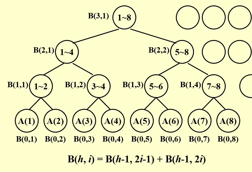
- \(\text{Depth}=O(\log N)\)
- \(\text{Work}=O(N)\)
3.1 PRAM Model#
| PRAM Model | |
|---|---|
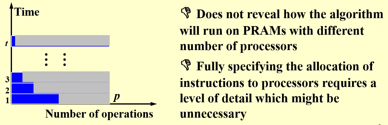
Bug
- 无法揭示算法和实际使用的处理器个数之间的关系
- 该模型需要指定哪个处理器处理哪部分的指令,这时就需要知道一些可能不太必要的细节,例如上面的
stay idle
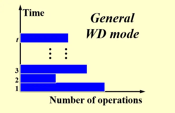
3.2 Work-Depth (WD) Presentation#
| WD Model | |
|---|---|
Tip
这里与 PRAM 不同,不再显式地指出每个处理器应该干什么
4 Performance Measurement#
- Work load \(W(n)\)
- Running time \(T(n)\)
4.1 PRAM#
- 将处理器个数与实际复杂度关联,其中的 \(T(n)\) 表示的是理想状态下(无限处理器个数)的 worst case time
- PRAM: \(P(n)=W(n)/T(n)\) processors and \(T(n)\) time
- PRAM: \(W(n)/p\) time using any number of \(p\leq W(n)/T(n)\) processors
- PRAM: \(W(n)/p+T(n)\) time using any number of \(p\) processors
- All asymptotically equivalent
4.2 WD#
Brent's Theorem
4.2.1 Discussion#
Question
Please prove that a parallel algorithm with workload \(W\) and depth \(D\) can be implemented in \(W/p+D\) time using \(p\) processors for any \(p>0\).
Assume that the workload on \(\text{depth}=i\) is \(w_{i}\).
In the worst case that each layer must be totally completed before executing any workload of the upper layer, we have \(t_{i}=\lceil w_{i}/p \rceil\), then:
5 Prefix Sums#
Question
求一个序列所有的 \(n\) 个前序和
可以借助求和问题:假设我们已经有了求和的树状结构和每个 node 的值 B[h, i],那么可以进一步求出 C[h, i] ,表示到其右叶子的前缀和
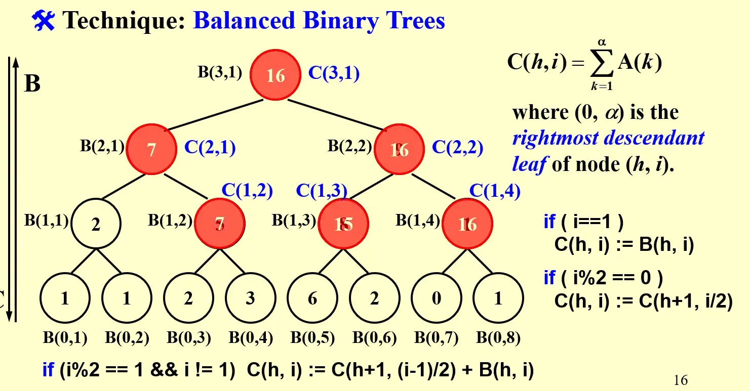
5.1 Implementation#
- 首先,左路径上
C[h, 1] = B[h, 1] - 其次,每一层的偶数节点都等于父节点
if (1 % 2 == 0) C[h, i] := C(h + 1, i / 2) - 最后,计算除了左路径外的所有奇数节点,相当于其左上方节点的值加上自己的 B 值
if (i % 2 == 0 && i != 1) C[h, i] := C[h+1, (i - 1) / 2] + B(h, i)
Note
top-down,每一层都可以并行计算
5.2 WD Analysis#
- \(T(N)=O(N \log N)\)
- Prefix Sum 和 Summation 是一样难的
- \(W(N)=O(N)\)
6 Merging#
将两个非递减的数组 \(A,B\) 合并到一个数组 \(C\)
进行下列简化
- \(A,B\) 元素不重复
- \(A,B\) 长度相等
- \(\log n,\frac{n}{\log n}\) 均为整数
6.1 Partition#
- 将较大的任务划分成很多独立的小任务
- 并行执行这些小任务
- 每个小任务用 serial algo 来解决
6.2 Ranking#
- \(\text{RANK}(j,A)\) 表示元素 \(j\) 在非递减的 \(A\) 中的插入位置索引
- 最终在 \(C\) 数组中的位置就是两个 RANK 之和
6.3 Ranking Methods#
6.3.1 并行二分查找#
- \(T(n)=O(\log n)\)
- \(W(n)=O(n\log n)\)
6.3.2 串行双指针#
- \(T(n)=O(m+n)\)
- \(W(n)=O(m+n)\)
6.3.3 Parallel Ranking#
假设 \(m=n\),而且 \(A(n+1), B(n+1)\) 都比 \(A(n),B(n)\) 大
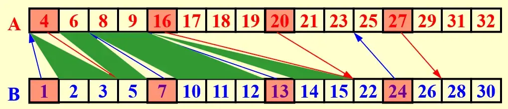
6.3.3.1 Stage 1: Partitioning#
- 假设有 \(p=n/\log n\) 个处理器
- 首先进行选择,以 \(\log n\) 为步长在两个数组中选择部分元素
- 然后对选中的元素进行排序 下图中的箭头标记了插入位置
- 转化成子问题 下图中部分标记为绿色
6.3.3.2 Stage 2: Actural Ranking#
最多得到 \(2p\) 个 \(O(\log n)\) 大小的子问题,分别进行串行排序
- \(W(n)=\frac{2n}{\log n} O(\log n)=O(n)\)
- \(T(n)=O(\log n)\)
7 Ultimate Parallel find_max#
| no. | type | \(T\) | \(W\) |
|---|---|---|---|
| a | serial | \(N\) | \(N\) |
| b | binary | \(\log N\) | \(N\) |
| c | pair-wise brute-force | \(1\) | \(N^2\) |
| d.1 | \(\log \log N\) | \(N\log \log N\) | |
| d.2 | \(\log \log N\) | \(N\) |
7.1 A Doubly-logarithmic Paradigm#
假设 \(h=\log \log n\) 是整数,\(n=2^{2^h}\)。
7.1.1 \(\sqrt{ n }\) partition d.1#
每一层都用 \(\sqrt{ n }\) 进行分治,那么在每一层的 conquer 开销为:
- \(T=C_{1}\)
- \(W=C_{2}n\)
那么有
所以 \(T(n)=O(\log \log n),\,W(n)=O(n\log \log n)\)。
7.1.2 \(h\)-partition d.2#
第一层先用 \(h\)-partition,后面还是 \(\sqrt{ n }\)-partition;那么第一层分过之后,有 \(n/h\) 个大小为 \(h\) 的子问题,每个子问题有 \(T=O(\log \log (n/h)),\,W=O((n/h)\log \log (n/h))\);最后再进行一个 \(T=O(h),\,W=O(h \cdot(n/h))\) 的 conquer:
7.1.3 Random Sampling d.3#
\(T=O(1),\,W=O(n)\), with very high probability, on an Arbitrary CRCW PRAM
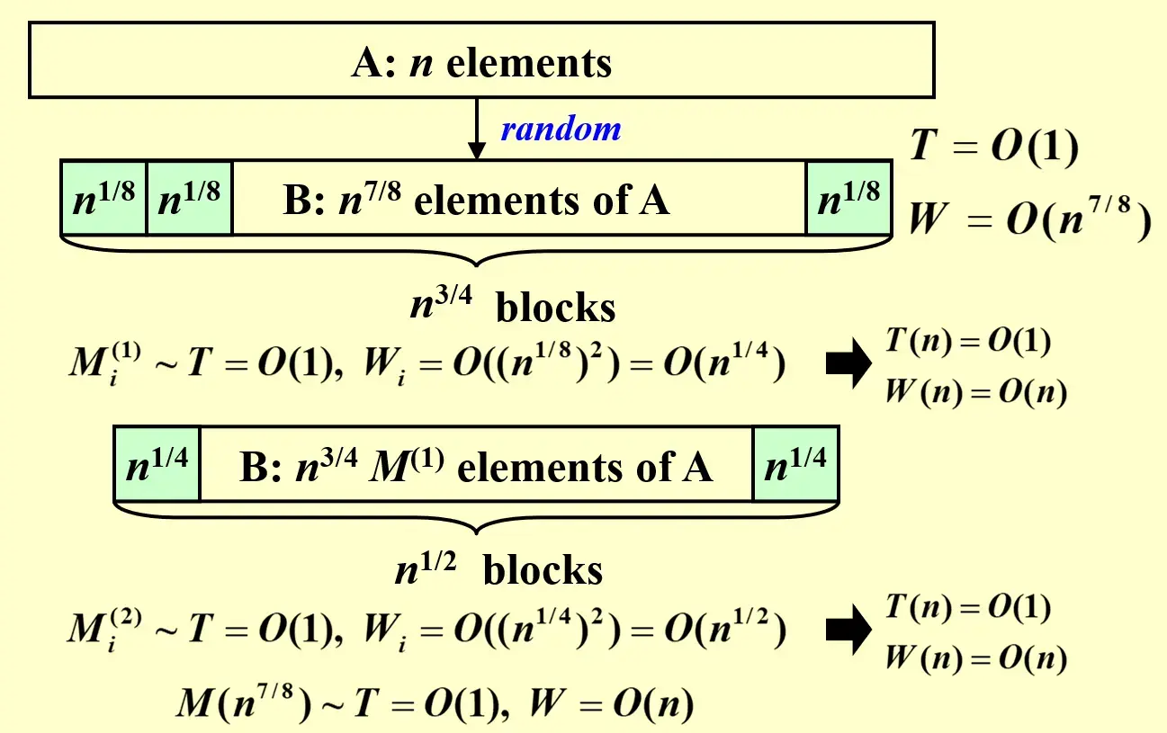
- 随机选择 \(n^{7/8}\) 个元素,分成 \(n^{3/4}\) 个大小为 \(n^{1/8}\) 的块
- \(T=O(1)\),可以并行选择
- \(W=O(n^{7/8})\)
- 对这 \(n^{3/4}\) 个块进行并行 maximum finding
- \(T=O(1)\)
- \(W_{i}=O(n^{1/4}), W=n^{3/4}O(n^{1/4})=O(n)\)
-
然后,让 \(n\) 个处理器拿着找到的最大值与原来的 \(n\) 个元素进行比较,如果原来的元素比这个大的话就随机写入到一个长度仍然为 \(n^{7/8}\) 的数组中,再进行一次,直到找到最大值
-
得到正确结果的概率相当大,失败的概率为 \(O(\frac{1}{n^c})\)
8 Questions#
8.1 HW14#
8.1.1 Merge-sort complexity#
Sorting-by-merging is a classic serial algorithm. It can be translated directly into a reasonably efficient parallel algorithm. A recursive description follows.
MERGE−SORT( A(1), A(2), ..., A(n); B(1), B(2), ..., B(n) )
Assume that \(n=2^l\) for some integer \(l\ge 0\)
if n = 1 then return B(1) := A(1)
else call, in parallel, MERGE−SORT( A(1), ..., A(n/2); C(1), ..., C(n/2) ) and
- MERGE−SORT(A(n/2+1), ..., A(n); C(n/2+1), ..., C(n) )
- Merge (C(1),...C(n/2)) and (C(n/2 + 1),...,C(n)) into (B(1), B(2), ..., B(n)) with time O(n)
Then the MERGE−SORT runs in __ .
Answer
Merge 一次的时间开销是 \(O(\log n)\),所以总体的时间开销应该是 \(O(\log^2 n)\) 题目中说 \(O(n)\) merge,但是这样的话早就 \(O(n)\) 了,估计是题目的问题
8.2 Q14#
8.2.1 W-D#
In Work-Depth presentation, each time unit consists of a sequence of instructions to be performed concurrently; the sequence of instructions may include any number. (T/F)
Answer
T, 定义就是这样说的,只要给定一个 unit 就行了,内部的操作数量任意