01 AVL Trees, Splay Trees and Amortized Analysis

1 AVL Trees: Self-Balancing Tree

• Target
  • 让二叉树的 height 尽量小
  • 减少 Average Search Time

1.1 Definition

• 空树平衡
• 非空树平衡当且仅当
  • 左右子树均平衡
  • 左右子树的高度相差 \(\le 1\)

Balance Factor \(BF(node) = h_L-h_R\)

1.2 Solution

• Trouble Maker: 插入之后导致不平衡的节点
• Trouble Finder: 探测到产生了不平衡的节点
• 四种调整情况：RR/LL LR/RL
  • 反映的是 Trouble finder 到 Trouble maker 的相对位置关系

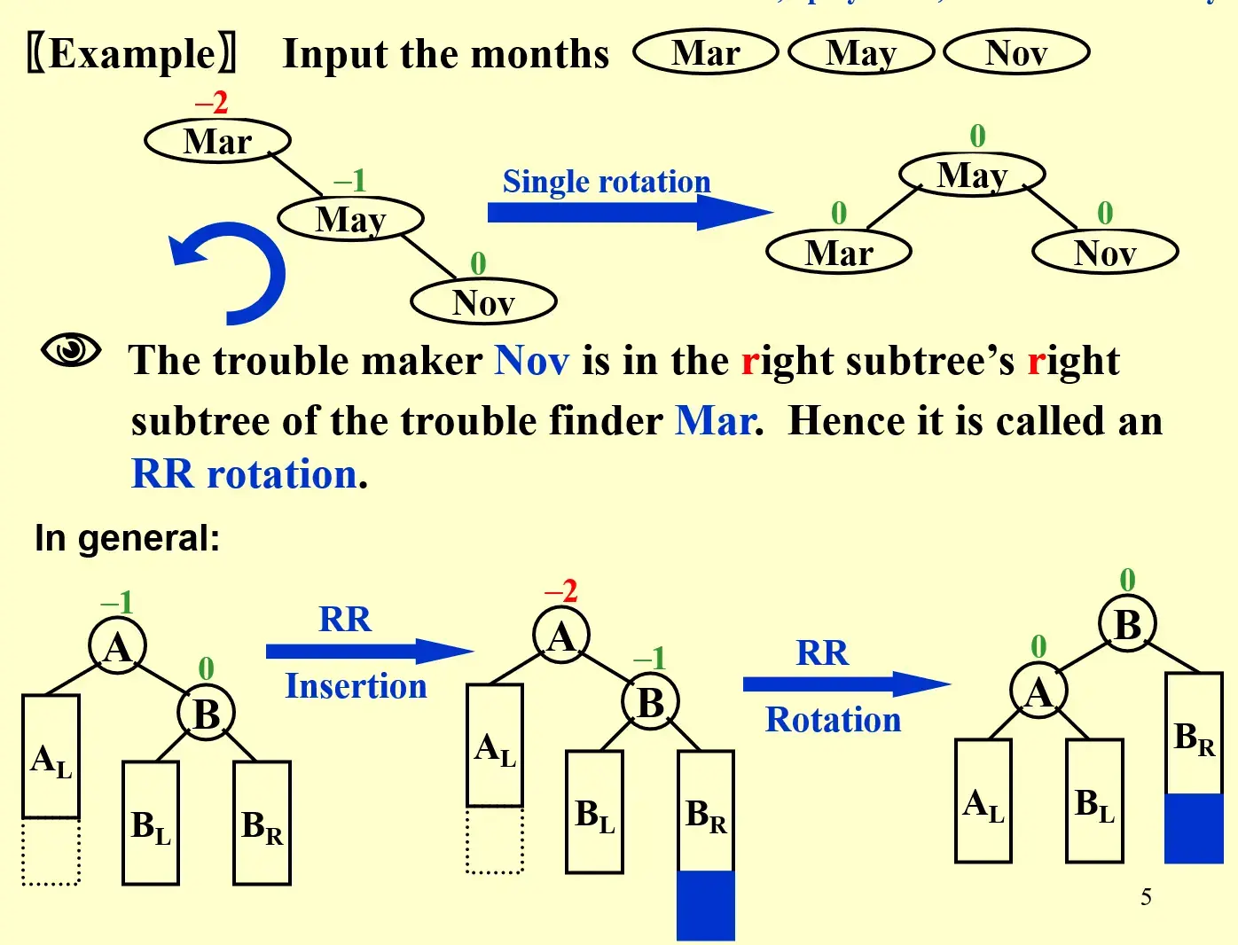
1.2.1 RR rotation

avl_ptr single_rotate_right(avl_ptr P){  // N is the rotation center
    avl_ptr N = P->right;
    P->right = N->left;
    N->left = P;
    P->height = max(height(P->right), height(P->left)) + 1;
    N->height = max(height(N->right), P->height) + 1;
    return N;
}

avl_ptr rr_rotate(avl_ptr trouble_finder){
    return single_rotate_right(trouble_finder);
}

rr_rotate(Mar);

1.2.2 rotation

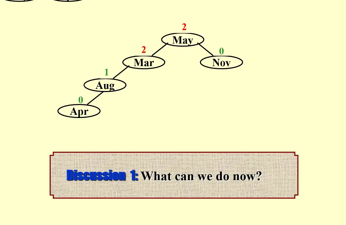
• 插入 Apr 后，发现 grandparent 产生了不平衡，于是需要对 Mar 进行 rotate

avl_ptr single_rotate_left(avl_ptr P){  // rotation to replace the parent node
    avl_ptr N = P->left;
    P->left = N->right;
    N->right = P;
    P->height = max(height(P->left), height(P->right)) + 1;
    N->height = max(height(N->left), P->height) + 1;
    return N;
}

avl_ptr ll_rotate(avl_ptr trouble_finder){  // first trouble finder
    return single_rotate_left(trouble_finder);
}

ll_rotate(Mar);

1.2.3 LR rotation

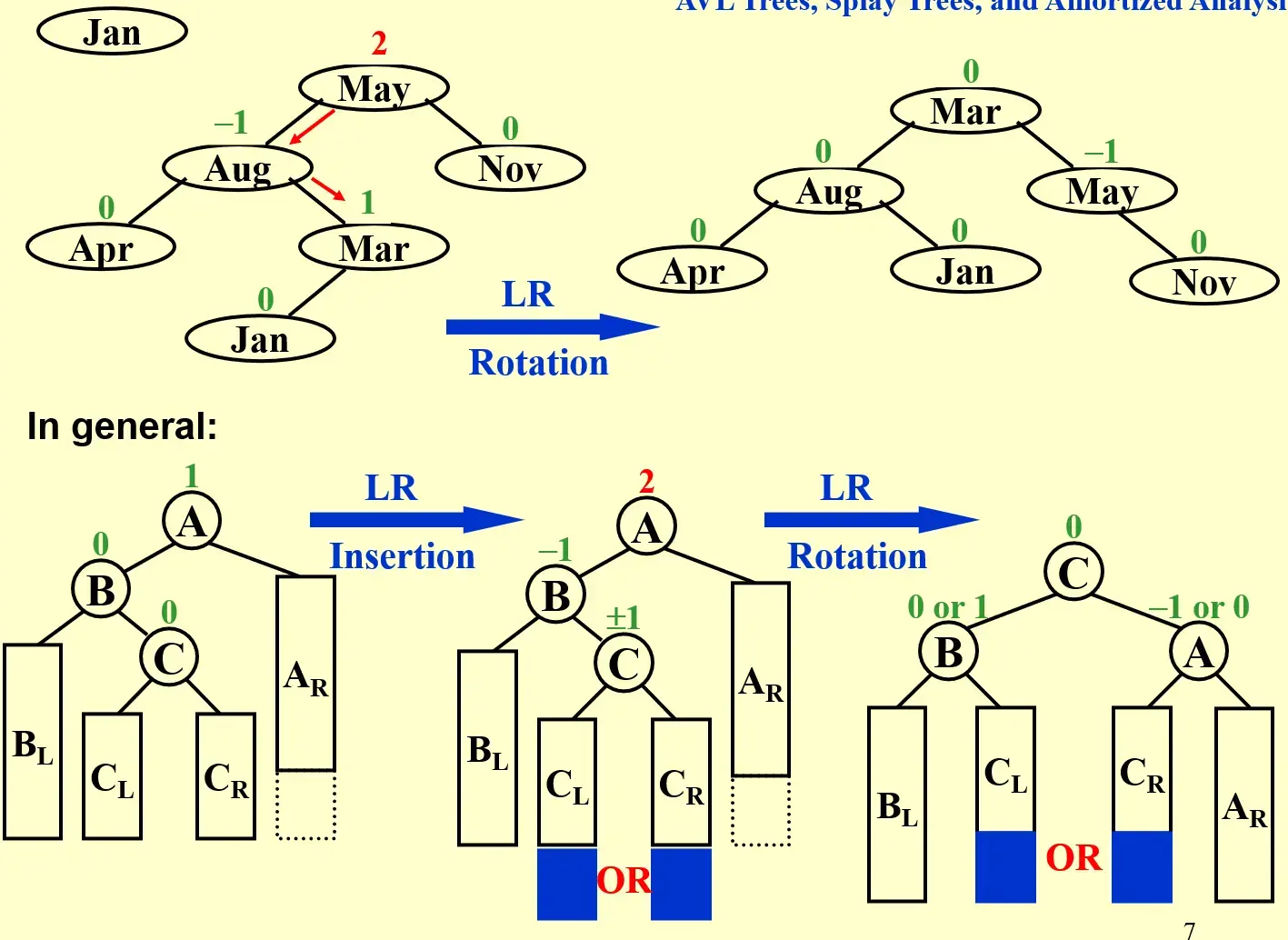
可以分成以下步骤

1. P 进行 single_rotate_right
2. G 进行 single_rotate_left，这里的 G 也就是 trouble_finder

avl_ptr lr_rotate(avl_ptr trouble_finder){
    trouble_finder->left = single_rotate_right(trouble_finder->left);
    return single_rotate_left(trouble_finder);
}

lr_rotate(May);

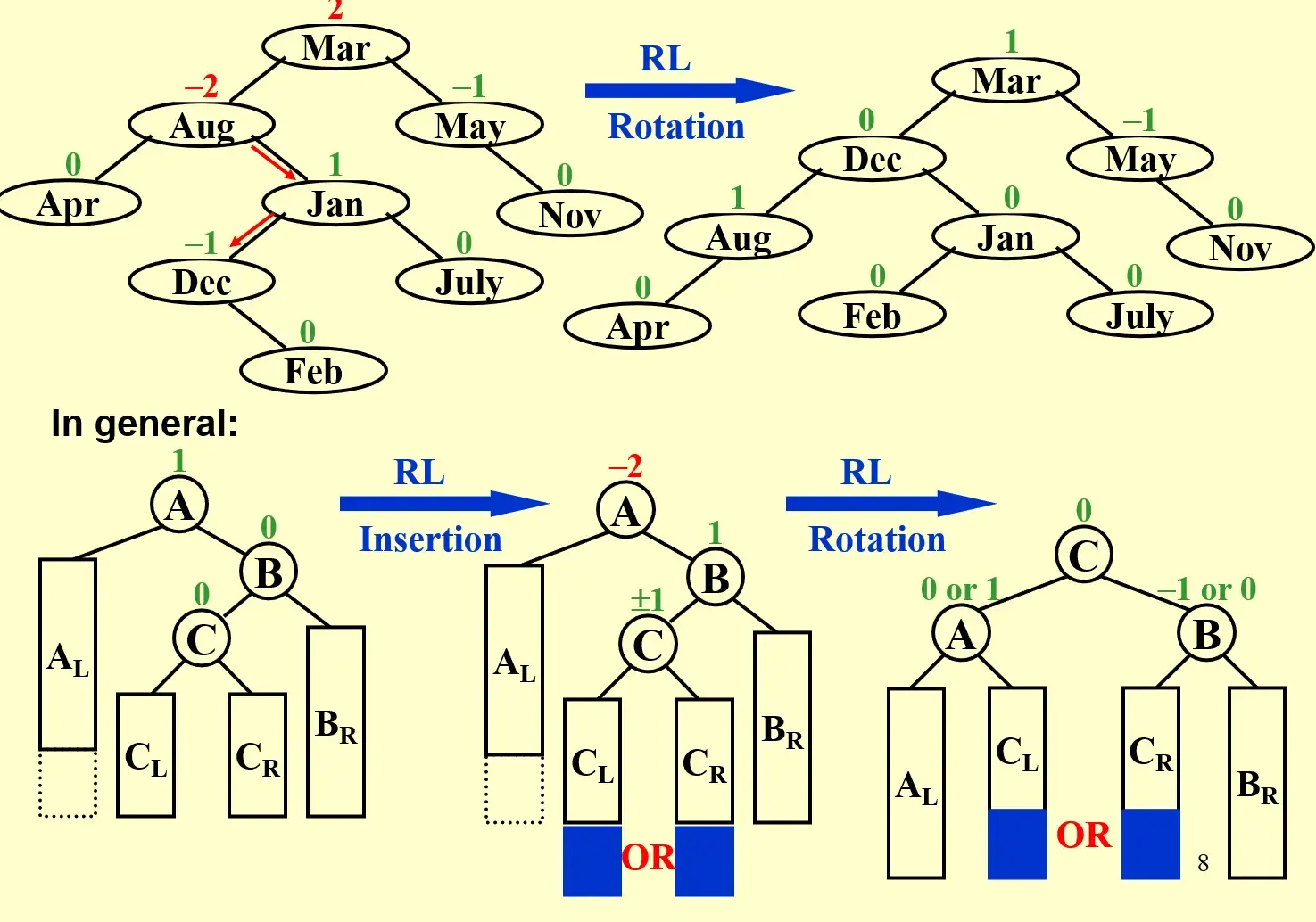
1.2.4 RL rotation

avl_ptr rl_rotate(avl_ptr trouble_finder){
    trouble_finder->right = single_rotate_left(trouble_finder->right);
    return single_rotate_right(trouble_finder->right);
}

rl_rotate(May);

总结

• 永远只找第一个 Trouble Finder，这也符合递归的遍历结构
• RR 和 LL 只用转一次，而 RL 和 LR 都需要转两次
• 为了维护树的结构，在 rotate 时需要记录 trouble_finder 的 parent（若有），并及时更新指针，single_rotate 函数均会返回 rotate 后的子树根节点，所以很好实现

1.3 One last question

给定 height 的 AVL Tree 的最少节点数：

\[ n_h=n_{h-1}+n_{h-2}+1 \]

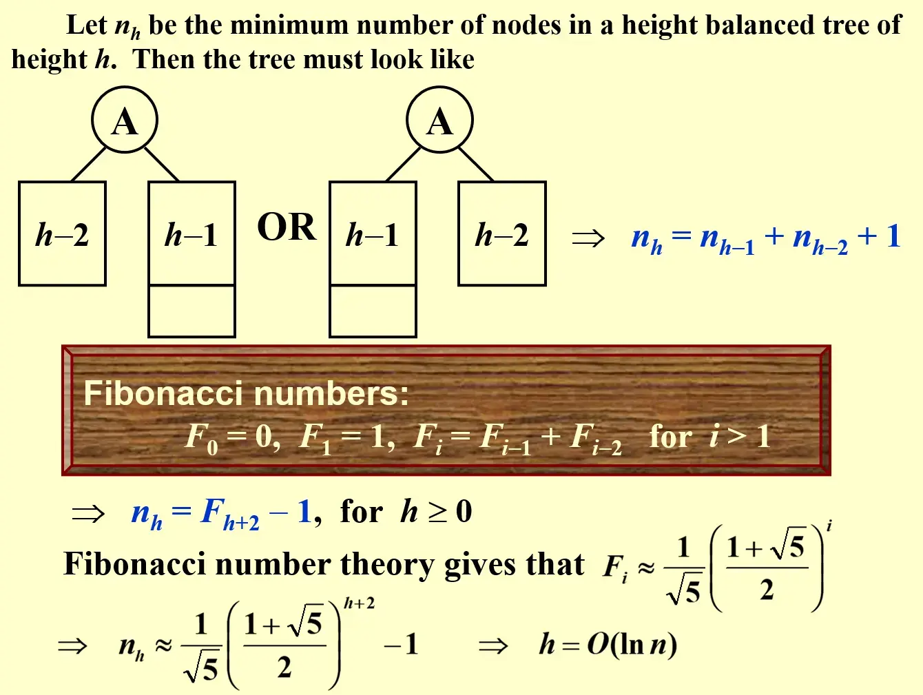
由此可以推导出：必记公式

\[ n_h=F_{h+3}-1 \]

也就是：

\[ \begin{align} n_h&\approx\frac{1}{\sqrt{5}}(\frac{1+\sqrt{5}}{2})^{h+3}-1 \\ \\ h&=O(\ln n) \end{align} \]

这说明了 AVL Tree 的平衡性。

Attention

课本中对 height 没有统一的定义，这里认为根节点的高度为 0，边才能提供高度

2 Splay Trees: Self-Adjusting Tree

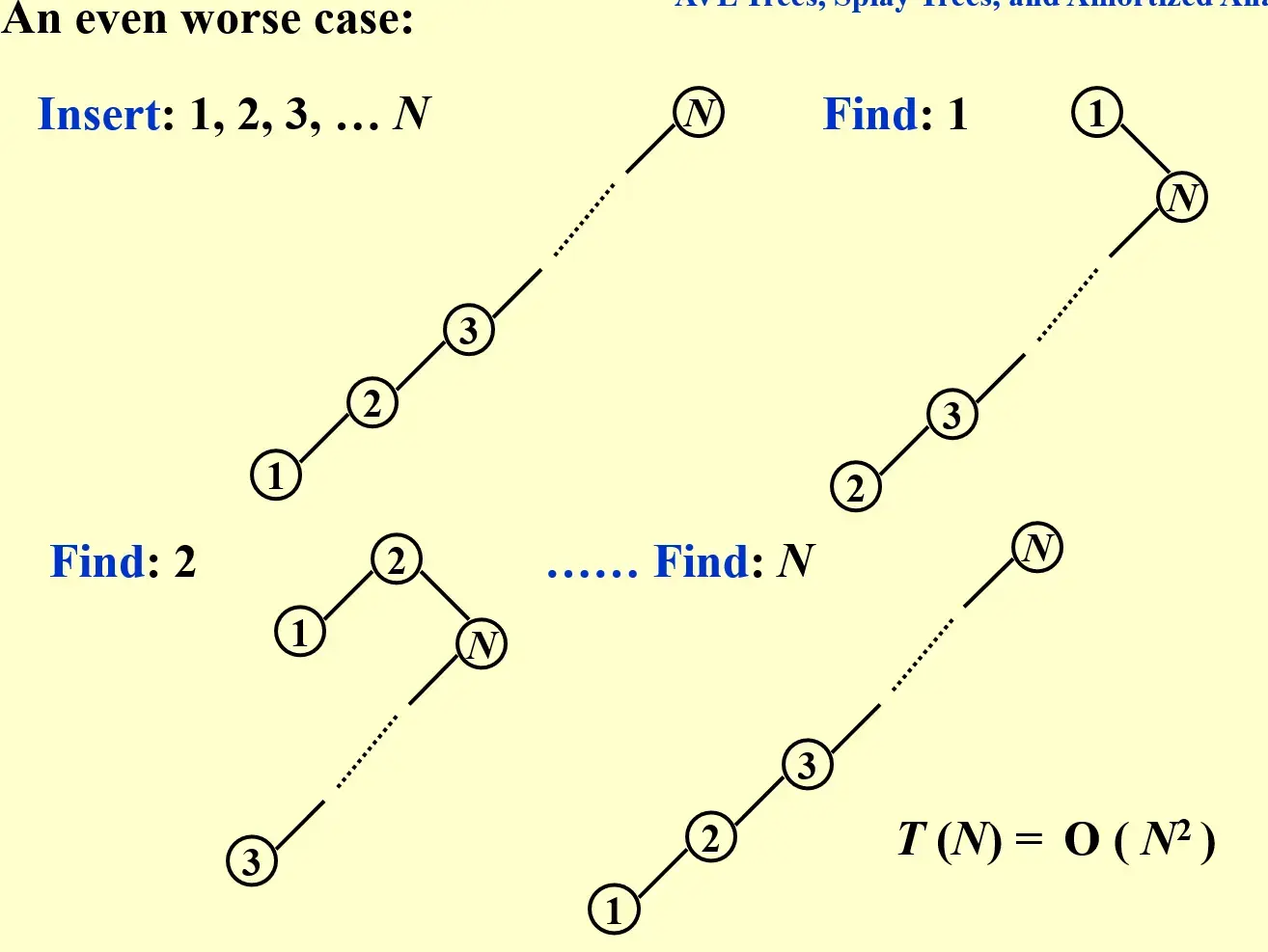
• Target: Any \(M\) consecutive tree operations starting from an empty tree take at most \(O(M\log N)\) time.
• 为了降低 amortized time，由于存在 \(O(N)\) 的访问请求，不能让这个请求每次都是 \(O(N)\)，所以要移动节点。
• 只要查询一个节点，就放到根上面去。

2.1 Amortized Time Complexity 均摊时间复杂度

• Worst Bound: \(W(C)=O(N)\)
  • 好算但没用
• Amoritzed Bound: \(A(C)=\sum_{i=1}^M c_i\)
  • 蒙特卡洛
  • 可计算、有意义
• Average Bound: \(E(C)=\int P(c) \cdot c dc\)
  • 有意义难计算

2.2 Solution

2.2.1 多次 single_rotate 为什么不行？

2.2.2 { Zig-zag, Zig-zig, Zig }

Attention

这里的 zig-zig 被认为是 single rotation，但事实上使用了两次 AVL rotations

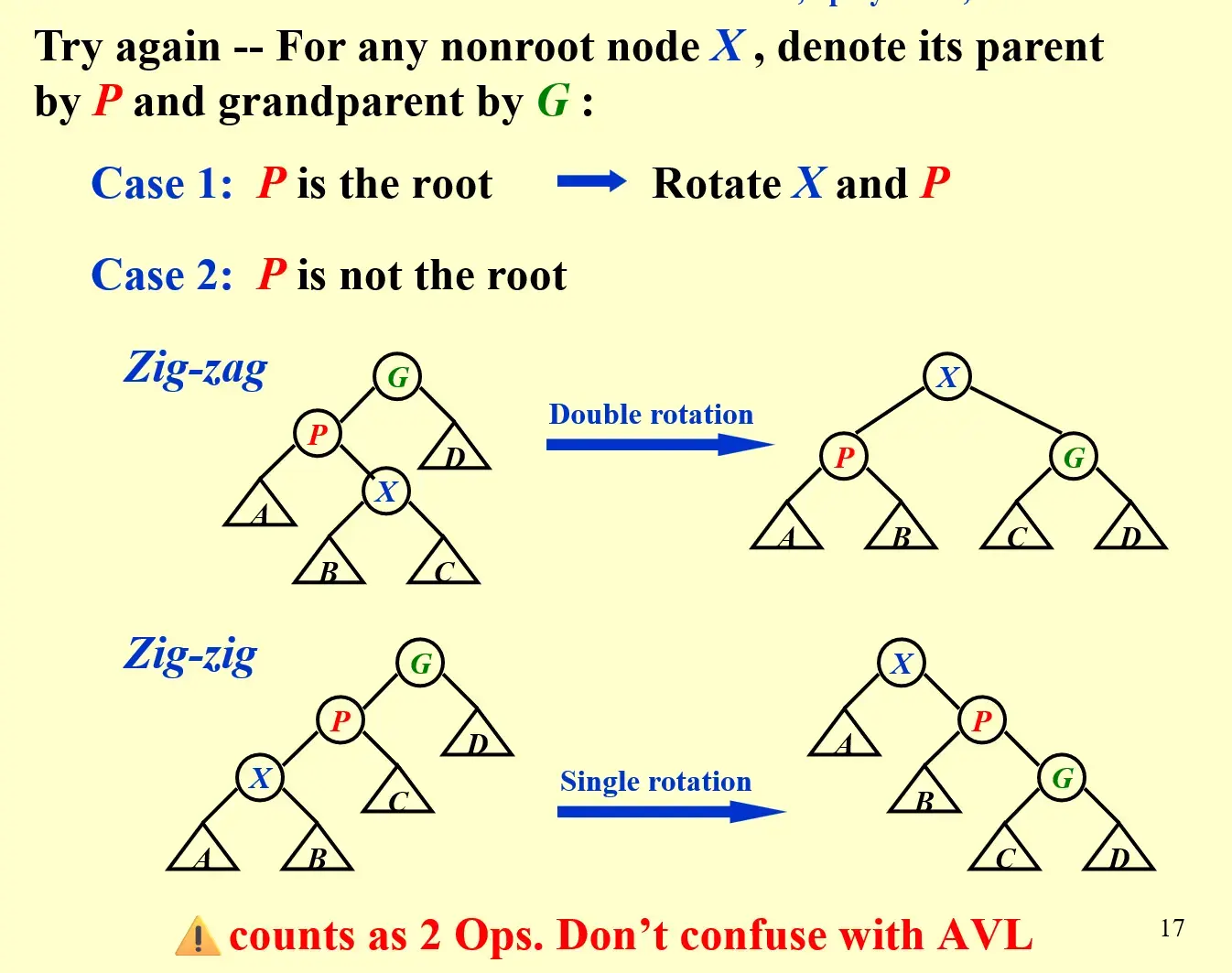
Hint

Splaying not only moves the accessed node to the root, but also roughly halves the depth of most nodes on the path. 所以 Splay Tree 也是平衡树

2.2.3 Insertion

1. Find 是否已经存在
   1. 如果不存在，按照 BST 插入
2. splay 这个元素所在的节点到根

2.2.4 Deletion

1. Find(x), x will be the root
2. Remove x, get 2 subtrees \(T_L\) and \(T_R\)
3. FindMax(\(T_L\)), max element will be the root
4. Make \(T_R\) the right child of the root of \(T_L\)

2.3 Advantage

• 存储空间小一些（不需要记录 \(BF\) ）

3 Amortized Analysis

Target: Any M consecutive operations take at most \(O(M\log N)\) time.

strength: worst-case bound \(\ge\) amortized bound Probablity not involved \(\ge\) average-case bound

Note

但是 amortized 结果可能比 average 要小

3.1 Aggregate analysis 聚合分析

对于所有 \(n\)，连续的 \(n\) 个操作总共花费的最坏时间为 \(T(n)\)，那么 amortized cost 为：

\[T_{amortized}=T(n)/n\]

3.1.1 e.g. Stach with MultiPop

从空栈开始连续进行 \(n\) 个 {push, pop, multiPop} 操作，有 \(sizeof(S)\le n\)。即使单次 MultiPop 可以是 \(O(sizeof(S))\)，但无法连续执行 \(O(n)\) 次，总复杂度不是 \(O(n^2)\) 而是 \(O(n)\)。每个被 push 的元素最多只能 pop 一次，所以

\[T_{amortized}=O(n)/n=O(1)\]

GPT 的解释

假设我们进行了一系列操作，包括多次 push、pop 和 multipop 操作。

• 每个 push 操作显然只需要 O(1) 的时间。
• 每个 pop 操作也需要 O(1) 的时间。
• 对于 multipop(k)，虽然它可能一次执行多次 pop，但重要的是，每个元素最多只能被弹出一次。因此，整个过程中无论是通过 pop 还是 multipop 弹出的元素，其数量最多为 n 次（即至多 n 个元素被压入栈并弹出）。

因此，即使 multipop(k) 在某次操作中可能执行 k 次 pop，但所有 pop 操作（包括在 multipop 中的）总共不会超过 n 次。

Aggregate Analysis 结论：

• 如果执行了 n 次操作（其中包括 push、pop 和 multipop 操作），那么总的时间复杂度是 O(n)。
• 于是每次操作的摊还复杂度是 O(1)。

3.2 Accounting method 核算法

Amortized cost \(\hat c_i\) 超过 actual cost \(c_i\) 的操作，可以 pay for 其他 \(\hat c_i < c_i\) 的操作，要保证摊还费用能够支付实际费用

\[ \begin{align} \sum_{i=1}^n \hat c_i \ge& \sum_{i=1}^n c_i \\ \\ T_{amoritzed}=&\frac{\sum_{i=1}^n \hat c_i}{n} \end{align} \]

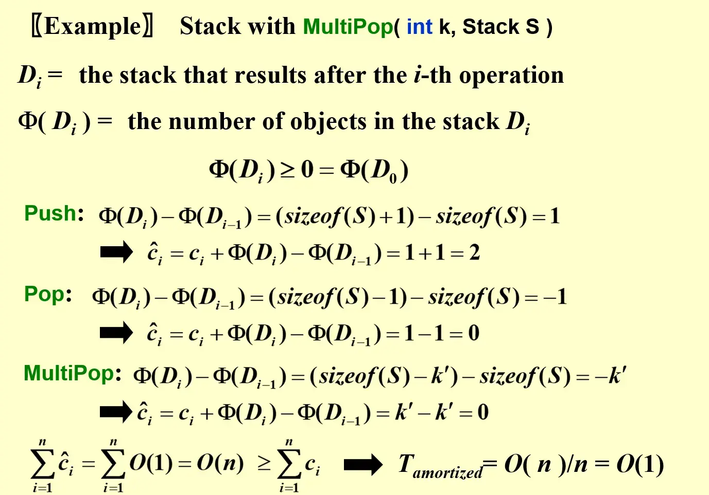
3.2.1 e.g. Stack with MultiPop

在 push 时分配 \(\hat c_i=2\) 来支付弹出时的花销，这样 pop 的摊还花销都是 \(\hat c_i=0\)，满足了

\[O(n)=\sum_{i=1}^n \hat c_i \ge \sum_{i=1}^n c_i\]

所以

\[T_{amoritzed}=\frac{\sum_{i=1}^n \hat c_i}{n}=\frac{O(n)}{n}=O(1)\]

3.3 Potential method 势能法

3.3.1 势能函数

势能函数的选择

选择势能函数时，核心原则是确保势能函数能够准确反映数据结构状态的变化，并能够帮助解释操作的摊还代价。在不同的问题中，势能函数的选择方式会有所不同，但通常会遵循以下几个指导原则：

1. 势能函数要与数据结构状态相关： 势能函数 \(\Phi\) 通常是数据结构的某些属性的函数。它应该能够反映操作前后系统状态的变化。常见的选择包括：

2. 数据结构中的元素数量。

3. 数据结构的某种“复杂度”指标，如堆的高度、队列的长度等。

4. 势能函数的变化应能解释操作的代价：

5. 当一个操作增加系统的复杂度时，势能应该相应增加，这意味着未来操作可能会减少这部分复杂度，势能可以用来支付高代价的操作。

6. 当一个操作降低系统复杂度时，势能应该减少，表明之前存储的“潜在开销”可以被利用，来减少当前操作的成本。

7. 确保势能函数非负： 为了使势能法的分析合理，势能函数必须始终是非负的。初始状态下的势能通常设置为零，随着操作的进行，势能可能会增加或减少，但总是保持非负。

8. 势能的总变化不能超过实际的代价总和： 选择势能函数时要确保，整个操作序列中的势能变化不会比实际的操作代价增长得更快。也就是说，势能的增加不能过度夸大操作的摊还代价。

\[ \begin{align} \hat c_i-c_i=&Credit_i=\Phi(D_i)-\Phi(D_{i-1}) \\ \\ \sum_{i=1}^n\hat c_i=&\sum_{i=1}^n(c_i+\Phi(D_i)-\Phi(D_{i-1}))=\sum_{i=1}^nc_i+\Phi(D_n)-\Phi(D_0) \end{align} \]

其中 \(\Phi(D_n)-\Phi(D_0)\ge 0\)

In general, a good potential function should always assume its minimum at the start of the sequence.

3.3.2 e.g. Stack with MultiPop

3.3.3 Splay Trees: \(T_{amortized}=O(\log N)\)

\[\Phi(T)=\sum_{i \in T} \log S(i)\]

其中 \(S(i)\) 表示以 \(i\) 为根节点的子树中节点数之和，这样，当树更加平衡时，势能较小。

考察三种 splay 操作的摊还花销：

zig

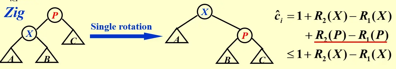
• \(c_i=1\)，因为只有一次旋转
• 势能函数中只有 X, P 两个节点的 rank 发生了变化，且 \(R(P)\) 变小所以可以放缩

zig-zag

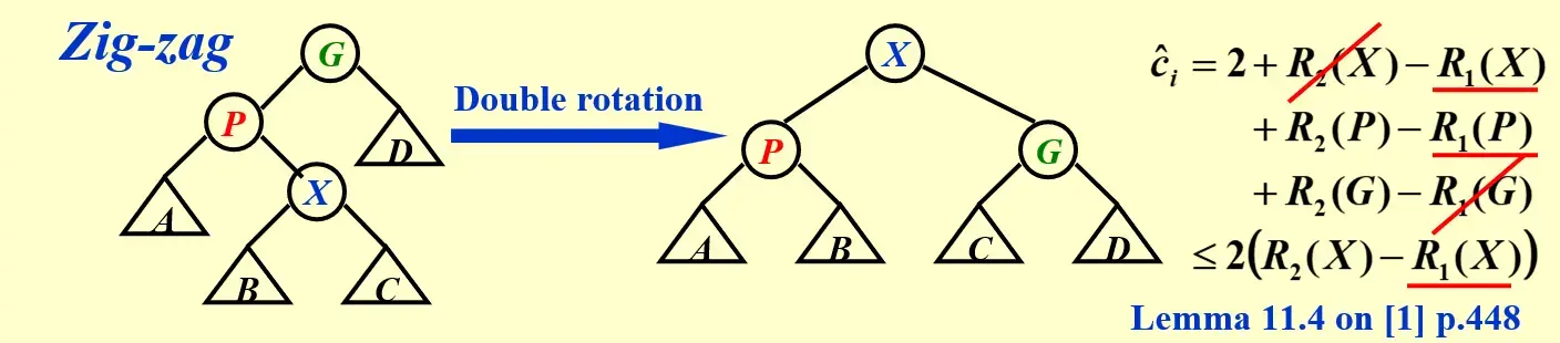
• \(c_i=2\)，因为实际旋转 2 次
• 同理，由于 \(R(P)\) 和 \(R(G)\) 都变小，可以放缩
• 进一步 X 一定至少多了两个后代 P, G，所以 \(R_2(X)-R_1(X)\ge 2\)，可以进一步放缩

zig-zig

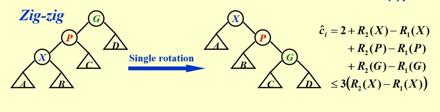
• \(c_i=2\)，因为实际旋转 2 次
• 同理，\(R(G)\) 一定减小，可以放缩掉
• \(R(P)\) 的变化情况不确定，但一定有 \(R_2(P)-R_1(P)\le R_2(X)-R_1(X)\)
• 且同理有 \(R_2(X)-R_1(X)\ge 2\)

综上，有 \(\hat c_i \le 1+3(R_2(X)-R_1(X))\)

The amortized time to splay a tree with root \(T\) at node \(X\) is at most \(3(R(T)-R(X))+1=O(\log N)\)

4 Questions

4.1 HW1

4.1.1 给定 AVL 树高，求最小节点数

If the depth of an AVL tree is 6 (the depth of an empty tree is defined to be -1), then the minimum possible number of nodes in this tree is:

Answer

\(n_h=F_{h+3}-1\) 必记公式

4.1.2 熟练进行 Splay

建议尝试一遍

4.1.3 选择合适的势能函数

Consider the following buffer management problem. Initially the buffer size (the number of blocks) is one. Each block can accommodate exactly one item. As soon as a new item arrives, check if there is an available block. If yes, put the item into the block, induced a cost of one. Otherwise, the buffer size is doubled, and then the item is able to put into. Moreover, the old items have to be moved into the new buffer so it costs k+1 to make this insertion, where k is the number of old items. Clearly, if there are N items, the worst-case cost for one insertion can be Ω(N). To show that the average cost is O(1), let us turn to the amortized analysis. To simplify the problem, assume that the buffer is full after all the N items are placed. Which of the following potential functions works? 参考 Homework - Jianjun Zhou's Notebook (zhoutimemachine.github.io)

• A. The number of items currently in the buffer
• B. The opposite number of items currently in the buffer
• C. The number of available blocks currently in the buffer
• D. The opposite number of available blocks in the buffer

Answer

D

• 设 \(size_i\) 为第 \(i\) 次插入前 buffer 的大小，则 \(\hat c_i=c_i+\Phi_i-\Phi_{i-1}\)。如果插入前 buffer 没满，\(c_i=1\)，否则 \(c_i=size_i\)

• 然后依次尝试每个选项，选择总是有 \(\hat c_i=O(1)\) 的

• 使用排除法

  • 首先，插入的时候势能一定要分摊掉，简单插入的势能肯定增加，排除 B C
  • 其次，在进行扩展的时候，势能一定能减少，来平均掉扩展的复杂度，A 势能 +1，D 才会减少，故选 D

Hint

直接套用势能函数到实际开销超过 O(1) 的操作上，然后检验是不是能摊还成 O(1)

4.1.4 编程题：AVL Tree 插入实现

Attention

• 由于本章节课件没有代码实现，可以借鉴课本上的代码
• 高度更新的时机十分重要

实现 AVL tree 的插入，并输出根节点元素。大部分代码源于课本，但修复了 bug

4.2 Ex1

4.2.1 Amortized bounds weaker/stronger?

Amortized bounds are weaker than the corresponding worst-case bounds, because there is no guarantee for any single operation. (T/F)

Answer

T 记住 Worst \(\geq\) Amortized \(\geq\) Average 就好了，大的就是 stronger

4.2.2 初始非零的势能函数

Suppose we have a potential function \(\Phi\) such that for all \(\Phi(D_{i})\geq \Phi(D_{0})\) for all \(i\), but \(\Phi(D_{0})\neq 0\). Then there exists a potential \(\Phi'\) such that \(\Phi'(D_{0})=0\), \(\Phi'(D_{i})\geq 0\) for all \(i\geq 1\), and the amortized costs using \(\Phi'\) are the same as the amortized costs using \(\Phi\). (T/F)

Answer

T，势能函数的初始值可以不是 0，其实就是定义一个势能零点，而且问的是存在 exist

4.2.3 AVL Tree 高度和节点数关系

The height of an AVL tree of 30 nodes can be 5. (The height of an empty tree is defined to be -1). (T/F)

Answer

T 根据公式直接求出高度为 5 的 AVL 的节点数范围，\([n_{5},2^{5+1}-1]=[F_{8}-1,63]=[20,63]\)

If there are 14 nodes in an AVL tree, then the maximum depth of the tree is ____. The depth of an empty tree is defined to be 0.

Answer

• 这里要注意，空树的高度不是 -1 而是 0，也就是说根节点的高度是 1
• 根据 \(n_{h}=F_{h+3}-1\) 得到最大的高度是 4，所以这里是 4+1=5

4.2.4 平衡树性质判断

Among the following 6 statements about AVL trees and splay trees, how many of them are correct?

(1) AVL tree is a kind of height balanced tree. In a legal AVL tree, each node's balance factor can only be 0 or 1.

(2) Define a single-node tree's height to be 1. For an AVL tree of height h, there are at most \(2^h−1\) nodes.

(3) Since AVL tree is strictly balanced, if the balance factor of any node changes, this node must be rotated.

(4) In a splay tree, if we only have to find a node without any more operation, it is acceptable that we don't push it to root and hence reduce the operation cost. Otherwise, we must push this node to the root position.

(5) In a splay tree, for any non-root node X, its parent P and grandparent G (guranteed to exist), the correct operation to splay X to G is to rotate X upward twice.

(6) Splaying roughly halves the depth of most nodes on the access path.

Answer

2 应该只有 (2) (6) 正确，(4) 不对，即使只是查找也要进行 splay，这是 Splay Tree 的定义

4.2.5 AVL Tree 插入操作

Insert { 9, 8, 7, 2, 3, 5, 6, 4 } one by one into an initially empty AVL tree. How many of the following statements is/are FALSE?

• the total number of rotations made is 5 (Note: double rotation counts 2 and single rotation counts 1)
• the expectation (round to 0.01) of access time is 2.75
• there are 2 nodes with a balance factor of -1

Answer

0 所有都正确，第一个差点算错 建议开始画图之前先看看有没有选项是和过程相关的

4.2.6 一些正误判断

Which one of the following statements is FALSE?

• A. For red-black trees, the total cost of rebalancing for m consecutive insertions in a tree of n nodes is \(O(n+m)\).
• B. To obtain \(O(1\)) armortized time for the function decrease-key, the potential function used for Fibonacci heaps is \(\Phi(H)=t(H)+m(H)\), where \(t(H)\) is the number of trees in the root list of heap \(H\), and \(m(H)\) is the number of marked nodes in \(H\).
• C. Let \(S(x)\) be the number of descendants of \(x\) (\(x\) included). If the potential function used for splay tree is \(\Phi(T)=\sum_{x \in T}​\log S(x)\) , then the amortized cost of one splay operation is \(O(\log n)\).
• D. In the potential method, the amortized cost of an operation is equal to the actual cost plus the increase in potential due to this operation.

Answer

B

• A. 旋转显然正确，染色的话每次染色都会增加一个黑色节点，不可能增加超过 \(O(m+n)\) 个黑色节点
• B. 斐波那契堆的势能函数通常是 \(\Phi(H)=t(H)+2m(H)\)
• C. 根据笔记，这是正确的
• D. 正确，是定义

4.3 Midterm

4.3.1 Splay tree 插入操作

Insert {3,9,6,1,8,7} into an initially empty splay tree, 7 is the parent of 6. (T/F)

Answer

T Splay tree 插入操作，先按照 BST 插入，然后 splay 到根节点

Comments